xobjmap

Xarray-native objective mapping and interpolation of scattered observations.

Rankine vortex reconstruction

Installation

With pip:

pip install xobjmap              # numpy only
pip install 'xobjmap[jax]'      # + JAX (CPU)
pip install 'xobjmap[jax-cuda]' # + JAX with GPU (CUDA 12)

With pixi (recommended for development):

pixi add xobjmap

Quick start

import numpy as np
import xarray as xr
import xobjmap

# Scattered observations
obs = xr.Dataset(
    {"temp": ("station", temp_data)},
    coords={"lon": ("station", lons), "lat": ("station", lats)},
)

# Target grid
target = xr.Dataset(
    coords={"lon": np.linspace(-40, -38, 50), "lat": np.linspace(-24, -22, 40)}
)

# Scalar objective analysis
result = obs.xobjmap.scalar(
    "temp", target, corrlen={"lon": 1.0, "lat": 0.5}, err=0.1
)
result.temp   # interpolated field
result.error  # normalized error map

# Streamfunction recovery
obs_vel = xr.Dataset(
    {"u": ("station", u_data), "v": ("station", v_data)},
    coords={"lon": ("station", lons), "lat": ("station", lats)},
)
result_psi = obs_vel.xobjmap.streamfunction(
    "u", "v", target, corrlen={"lon": 1.0, "lat": 0.5}, err=0.1
)
result_psi.psi
result_psi.psi_error

# Velocity potential recovery
result_chi = obs_vel.xobjmap.velocity_potential(
    "u", "v", target, corrlen={"lon": 1.0, "lat": 0.5}, err=0.1
)
result_chi.chi
result_chi.chi_error

# Helmholtz decomposition
result = obs_vel.xobjmap.helmholtz(
    "u", "v", target,
    corrlen_psi={"lon": 1.0, "lat": 0.5},
    corrlen_chi={"lon": 1.0, "lat": 0.5},
    err=0.1,
)
result.psi
result.chi
result.psi_error
result.chi_error

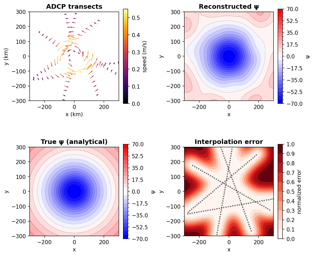
Example: ADCP Transects Through a Simple Helmholtz Flow

The example script examples/adcp_convergent_vortices.py builds synthetic ship ADCP transects across a simple theoretical flow made from:

a Gaussian streamfunction psi that generates a non-divergent vortex
a Gaussian velocity potential chi that generates a non-rotational convergent feature
current speed used for scalar objective mapping

It compares the classic Bretherton direct solve (backend="numpy") and the JAX backend for both scalar mapping and Helmholtz recovery.

Run it with:

pixi run -e docs python examples/adcp_convergent_vortices.py

ADCP Helmholtz flow comparison

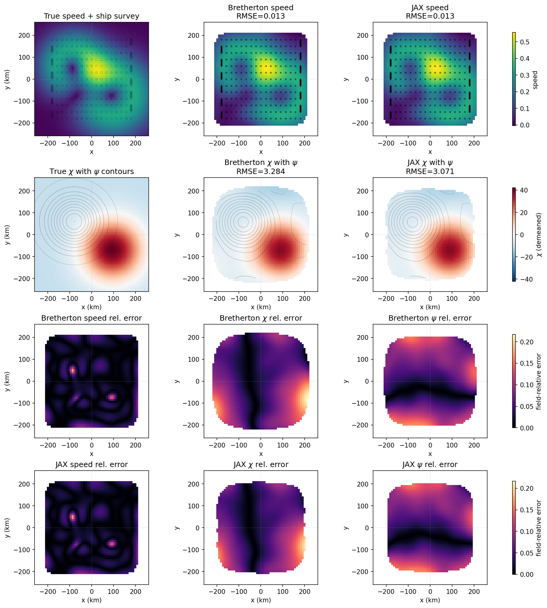
The ship survey is confined to a narrower [-180, 180] footprint in both x and y, which makes the edge uncertainty more visible. The first row compares the true speed field sampled along the ship survey against scalar reconstructions using a shared row colorbar. The second row shows the true velocity potential chi with streamfunction psi contours, followed by the Helmholtz reconstructions with a shared row colorbar. The third row shows the Bretherton field-relative errors for speed, chi, and psi, and the fourth row shows the corresponding JAX field-relative errors. These are normalized by each true field's peak magnitude so the panels remain comparable despite their different units. The reconstructed panels mask mapped values where the normalized posterior error exceeds a fixed threshold, using a stricter cutoff for speed than for the Helmholtz potential fields so that psi and chi remain visible.

Benchmarking

For large 3-D Helmholtz backend comparisons, use:

pixi run -e test-jax-cuda python examples/benchmark_helmholtz_3d.py

This benchmark targets the accessor N-D Helmholtz path with interp_dims=('x', 'y', 'z') and derivative_dims=('x', 'y'), and defaults to comparing dense NumPy against JAX on CUDA.

Examples:

pixi run -e test-jax-cuda python examples/benchmark_helmholtz_3d.py \
  --sizes 900 1400 2000 --nx 80 --ny 80 --nz 3

pixi run -e test-jax-cuda python examples/benchmark_helmholtz_3d.py \
  --sizes 1000 3000 10000 --nx 100 --ny 100 --nz 5

pixi run -e test-jax-cuda python examples/benchmark_helmholtz_3d.py \
  --backends jax-gpu --sizes 2000 3000 4000 6000

The dense NumPy memory estimate printed by the benchmark is a lower bound for the dominant arrays, not a full process-memory prediction. Real NumPy RSS can be substantially larger because of temporaries, solve workspace, and allocator overhead.

Results can also be written to JSON or CSV:

pixi run -e test-jax-cuda python examples/benchmark_helmholtz_3d.py \
  --sizes 900 1400 2000 --json /tmp/helmholtz3d.json --csv /tmp/helmholtz3d.csv

API Reference

Accessor methods

`ds.xobjmap.scalar(var, target, corrlen, err, backend="numpy", return_error=True, k_local=None)`

Interpolates a scalar variable from scattered observations onto target locations.

Parameter	Type	Description
`var`	`str`	Variable name in the dataset
`target`	`xr.Dataset`	Target coordinates
`corrlen`	`dict` or `float`	Correlation length scales (same units as coordinates)
`err`	`float`	Normalized error variance (0 to 1)
`return_error`	`bool`	If `True`, also compute and return the error field
`k_local`	`int` or `None`	Local neighborhood size for JAX error estimates

Returns an xr.Dataset with the interpolated field and an error variable.

`ds.xobjmap.scalar_error(target, corrlen, err, backend="numpy", k_local=None)`

Returns only the scalar interpolation error field for the target grid.

`ds.xobjmap.streamfunction(u_var, v_var, target, corrlen, err, b=0, backend="numpy", return_error=True, k_local=None)`

Recovers the streamfunction from scattered velocity observations, assuming purely nondivergent flow.

Parameter	Type	Description
`u_var`	`str`	Eastward velocity variable name
`v_var`	`str`	Northward velocity variable name
`target`	`xr.Dataset`	Target grid coordinates
`corrlen`	`dict` or `float`	Correlation length scales (same units as coordinates)
`err`	`float`	Normalized error variance (0 to 1)
`b`	`float`	Mean correction parameter (default: 0)
`return_error`	`bool`	If `True`, also compute and return `psi_error`
`k_local`	`int` or `None`	Local neighborhood size for JAX error estimates

Returns an xr.Dataset with psi and, by default, psi_error.

`ds.xobjmap.streamfunction_error(u_var, v_var, target, corrlen, err, b=0, backend="numpy", k_local=None)`

Returns only the streamfunction posterior error field.

`ds.xobjmap.velocity_potential(u_var, v_var, target, corrlen, err, b=0, backend="numpy", return_error=True, k_local=None)`

Recovers the velocity potential from scattered velocity observations, assuming purely irrotational flow.

Parameter	Type	Description
`u_var`	`str`	Eastward velocity variable name
`v_var`	`str`	Northward velocity variable name
`target`	`xr.Dataset`	Target grid coordinates
`corrlen`	`dict` or `float`	Correlation length scales (same units as coordinates)
`err`	`float`	Normalized error variance (0 to 1)
`b`	`float`	Mean correction parameter (default: 0)
`return_error`	`bool`	If `True`, also compute and return `chi_error`
`k_local`	`int` or `None`	Local neighborhood size for JAX error estimates

Returns an xr.Dataset with chi and, by default, chi_error.

`ds.xobjmap.velocity_potential_error(u_var, v_var, target, corrlen, err, b=0, backend="numpy", k_local=None)`

Returns only the velocity-potential posterior error field.

`ds.xobjmap.helmholtz(u_var, v_var, target, corrlen_psi, corrlen_chi, err, b=0, backend="numpy", return_error=True, k_local=None)`

Helmholtz decomposition: jointly recovers the streamfunction and velocity potential from scattered velocity observations.

Parameter	Type	Description
`u_var`	`str`	Eastward velocity variable name
`v_var`	`str`	Northward velocity variable name
`target`	`xr.Dataset`	Target grid coordinates
`corrlen_psi`	`dict` or `float`	Correlation length scales for the streamfunction
`corrlen_chi`	`dict` or `float`	Correlation length scales for the velocity potential
`err`	`float`	Normalized error variance (0 to 1)
`b`	`float`	Mean correction parameter (default: 0)
`return_error`	`bool`	If `True`, also compute and return `psi_error` and `chi_error`
`k_local`	`int` or `None`	Local neighborhood size for JAX error estimates

Returns an xr.Dataset with psi, chi, and, by default, psi_error and chi_error.

`ds.xobjmap.helmholtz_error(u_var, v_var, target, corrlen_psi, corrlen_chi, err, b=0, backend="numpy", k_local=None)`

Returns only the Helmholtz posterior error fields psi_error and chi_error.

Low-level functions

All low-level functions accept backend="jax" for lower memory usage and optional GPU acceleration.

`xobjmap.scalar(xc, yc, x, y, t, corrlenx, corrleny, err, backend="numpy")`

Scalar Gauss-Markov estimation. Returns the interpolated field tp.

`xobjmap.scalar_error(xc, yc, x, y, corrlenx, corrleny, err, backend="numpy", k_local=None)`

Scalar interpolation error field. Returns normalized mean squared error ep. Depends only on observation geometry, not on the observed scalar values. The JAX backend uses a local neighborhood approximation (k_local nearest observations per target point).

`xobjmap.streamfunction_error(xc, yc, x, y, corrlenx, corrleny, err, b=0, backend="numpy", k_local=None)`

Posterior error field for streamfunction recovery. Depends only on geometry, not on observed velocities.

`xobjmap.streamfunction(xc, yc, x, y, u, v, corrlenx, corrleny, err, b=0, backend="numpy")`

Recovers the streamfunction on the target grid (xc, yc), assuming nondivergent flow.

`xobjmap.velocity_potential_error(xc, yc, x, y, corrlenx, corrleny, err, b=0, backend="numpy", k_local=None)`

Posterior error field for velocity-potential recovery. Depends only on geometry, not on observed velocities.

`xobjmap.velocity_potential(xc, yc, x, y, u, v, corrlenx, corrleny, err, b=0, backend="numpy")`

Recovers the velocity potential on the target grid (xc, yc), assuming irrotational flow.

`xobjmap.helmholtz_error(xc, yc, x, y, corrlenx_psi, corrleny_psi, corrlenx_chi, corrleny_chi, err, b=0, backend="numpy", k_local=None)`

Posterior error fields for Helmholtz recovery. Returns (psi_error, chi_error). Depends only on geometry, not on observed velocities.

`xobjmap.helmholtz(xc, yc, x, y, u, v, corrlenx_psi, corrleny_psi, corrlenx_chi, corrleny_chi, err, b=0, backend="numpy")`

Helmholtz decomposition. Returns (psi, chi) on the target grid.

Notes

Correlation lengths must be in the same units as the coordinates. If working with lon/lat in degrees, either express corrlen in degrees or convert to a projected coordinate system first.
The streamfunction convention follows Bretherton et al. (1976): u = -dpsi/dy, v = dpsi/dx.
The velocity potential convention: u = dchi/dx, v = dchi/dy.
Error fields are normalized posterior uncertainties, not absolute physical-unit errors.
Scalar error and potential-field error are different inverse problems and should not be compared as if they were the same quantity.
The NumPy backend uses the direct dense Bretherton solve.
The JAX backend computes fields with a matrix-free conjugate-gradient solve and avoids global dense observation-covariance assembly.
JAX error fields use local-neighborhood solves (k_local) rather than global dense posterior solves, so JAX errors should be close to, but not expected to exactly match, the NumPy direct solution.

References

Bretherton, F. P., Davis, R. E., & Fandry, C. B. (1976). A technique for objective analysis and design of oceanographic experiments applied to MODE-73. Deep-Sea Research, 23(7), 559-582.